Dimension Reduction with Principal Component Analysis (PCA)

Here, in this post, we’ll see how to perform Dimension Reduction with Principal Component Analysis (PCA) using Sklearn library and also learn basic idea about dimension reduction and Principal Component Analysis (PCA).

Data is everywhere. Whatever you do in your day to day life will generate a tremendous amount of data that can be used by business to improve their products, to offer you better and relevant services. In fact, 90% of the data in the world has been generated in the last 4 years. Few examples of the kind of data being generated by you:

• Google collects data related to your demographics, interests to show relevant ads
• Social Networking websites like Facebook, Twitter collects data of what you like or love, share/retweet, post/tweet and even your location
• Smartwatches that you use collects data like distance covered, your heart rate, amount of calories burned etc.
• Online Marketplace like Amazon, Flipkart collects data of what you buy, view, click, etc. when you visit their website to recommend you a product or a list of products

As data generation and collection keeps increasing, getting an insight from that becomes more and more challenging. One of the easy ways of getting an insight from data is via visualization in form of charts/plots. For example, let’s say you have a dataset of a shape 1000 (rows/observations) and 50 (columns/features). So considering this dataset more than 1000 plots are possible to analyze the relationships. (In general, no. of plots drawn from a dataset with p features will be equal to p(p-1)/2 ). So you can think of how much time consuming it will be if you analyze and perform the exploratory analysis?

But not only the data but the features in the data are also increasing. Basically, datasets with a large number of features are called high-dimensional datasets.

If there are a lot of features in your dataset it will affect in both ways i.e. time taken to train a model as well as the accuracy of machine learning models. There are various ways by which we can reduce the features variables in our data. Here is a list below:

• Removing features with more number of missing values in a dataset
• Dropping low variance features from a dataset
• Keeping features which are highly correlated with the target or dependent variable.
• Principal Component Analysis (PCA)

Apart from these, there are other ways as well but for this post, we will see how to perform Dimension Reduction with Principal Component Analysis (PCA).

Dimension Reduction Technique

Dimension Reduction Technique can be defined as a technique which helps us in finding a pattern in data and uses these patterns to re-express it in a compressed form. During compression, only important and informative features are extracted and saved while less informative features also called noise features are removed. 

Let’s take an example, below is a chart showing temperature in Celsius and Fahrenheit.

Here, both variables are showing the same information. So, it would make sense to use only one variable. Simply, we can convert the data from 2D to 1D.

So in nutshell, by using dimensionality reduction, we can represent the same data using fewer features i.e. reduce p dimensions of the data into a subset of k dimensions (k<<p).

Principal Component Analysis (PCA)

The most fundamental of dimension reduction technique is Principal Component Analysis. It is used to transform high-dimensional datasets into a dataset with fewer features (or to transform a dataset into low dimension), where the remaining features explain the maximum variance within the dataset. It is called Principal Component Analysis because it learns from the ‘Principal Components’ of the data.

Principal Component Analysis aka PCA performs dimension reduction in two steps:

In the first step, it performs decorrelation which will not reduce the dimension but it will rotate the data samples so that they are aligned with the coordinate axis and the resulted samples or features are not linear correlated. Also, it will shift the data samples so that they have zero mean.

In the second step, it will reduce dimension.

Advantages of Dimension Reduction with Principal Component Analysis (PCA)

Here is a list of few main reasons and advantages of Dimension Reduction:

• If features in datasets are reduced, so the space required to store the data will be also less.
• Fewer features in the dataset will lead to less computation time and ultimately speed up machine learning algorithms
• Some algorithms perform well in lower dimensions
• It also helps to avoid multicollinearity issue by removing unnecessary features.
• It helps in visualizing all of the data clearly as discussed above.

Dimension Reduction with Principal Component Analysis (PCA)

Importing necessary modules

import pandas as pd
import numpy as np
import matplotlib.pyplot as plt
import seaborn as sns
from sklearn.model_selection import train_test_split
from sklearn.decomposition import PCA
from sklearn.preprocessing import StandardScaler
from sklearn.linear_model import LinearRegression
from sklearn.metrics import mean_squared_error

Read the Dataset

data = pd.read_csv("C:\\Users\\Pankaj\\Desktop\\Dataset\\Boston_housing.csv")

Print first 5 rows

data.head()

Missing Value

Generally, NaN or missing values can be in any form like 0, ? or may be written as “missing ” and in our case, as we can see above there are a lot of  0’s, so we can replace them with NaN to calculate how much data we are missing.

data.zn.replace(0, np.nan, inplace=True)
data.chas.replace(0, np.nan, inplace=True)

After replacing let’s again use .info() method to see the details about missing values in our dataset:

data.info()
Output-
<'pandas.core.frame.DataFrame'>
RangeIndex: 506 entries, 0 to 505
Data columns (total 14 columns):
crim 506 non-null float64
zn 134 non-null float64
indus 506 non-null float64
chas 35 non-null float64
nox 506 non-null float64
rm 506 non-null float64
age 506 non-null float64
dis 506 non-null float64
rad 506 non-null int64
tax 506 non-null int64
ptratio 506 non-null float64
b 506 non-null float64
lstat 506 non-null float64
medv 506 non-null float64
dtypes: float64(12), int64(2)
memory usage: 55.4 KB

Let’s calculate the percentage of missing values in our dataset. Generally, if there is 20-25% missing values we can impute them with different ways like mean, median or an educated guess by us. But if it’s more than that, it’s better to remove those features otherwise they can affect our result. As we can see below both “zn” and “chas” missing more than 70% data so we will remove both these features.

data.isnull().sum()/len(data)*100
Output-
crim 0.000000
zn 73.517787
indus 0.000000
chas 93.083004
nox 0.000000
rm 0.000000
age 0.0000<00
dis 0.000000
rad 0.000000
tax 0.000000
ptratio 0.000000
b 0.000000
lstat 0.000000
medv 0.000000
dtype: float64

We can drop both columns as shown below:

data = data.drop("zn", 1)
data = data.drop("chas", 1)

Finding Correlation between features and the target variable

data.corr()

 

Finding Correlation between Features and Target Variable in Boston Housing Dataset using Heatmap

correlation = data.corr()
plt.figure(figsize=(10,10))
sns.heatmap(correlation, vmax=1, square=True,annot=True,cmap='viridis')
plt.title('Correlation')

Observations from the above Heatmap and data.corr():

• From the above correlation plot, we can see that MEDV is strongly correlated to LSTAT, RM
• RAD and TAX are strongly correlated, so we don’t include this in our features together to avoid multicollinearity. Similar to the features DIS and AGE which have a correlation of -0.75. So we will exclude these four features from our features list.  You can find the reason behind this here.

Dropping Columns

data = data.drop(["rad","tax","dis","age"], 1)
data.shape
Output-
(506, 8)

Selecting Features and Target Variable

As Scikit learn wants “features” and “target” variables in X and y respectively. Here medv is our target variable, we can extract features and target arrays from our dataset as shown below. From X we drop the medv column along with other features and in y we keep only medv column:

X = data.drop(["medv", 1).values 
y= data["medv"].values

Instantiate Principal Component Analysis

Instantiating Principal Component Analysis as shown below:

pca = PCA()

Instantiate StandardScaler and use .fit() and .transform() methods

As PCA performs best with a normalized feature set. We must make sure that we standardize the data by transforming it onto a unit scale (mean=0 and variance=1).

scaler = StandardScaler()
X=scaler.fit_transform(X)
print(X)
Output-
array([[-0.41978194, -1.2879095 , -0.14421743, ..., -1.45900038,
         0.44105193, -1.0755623 ],
       [-0.41733926, -0.59338101, -0.74026221, ..., -0.30309415,
         0.44105193, -0.49243937],
       [-0.41734159, -0.59338101, -0.74026221, ..., -0.30309415,
         0.39642699, -1.2087274 ],
       ...,
       [-0.41344658,  0.11573841,  0.15812412, ...,  1.17646583,
         0.44105193, -0.98304761],
       [-0.40776407,  0.11573841,  0.15812412, ...,  1.17646583,
         0.4032249 , -0.86530163],
       [-0.41500016,  0.11573841,  0.15812412, ...,  1.17646583,
         0.44105193, -0.66905833]])

Now use .fit_transform() method of pca on features as shonw below:

pca.fit_transform(X)
Output-
array([[-1.97211024,  0.59768267, -0.60108255, ...,  0.38664927,
         0.28142543, -0.62304466],
       [-1.23831918, -0.25830272,  0.06828658, ...,  0.05618521,
         0.02647495,  0.09980334],
       [-1.91503575,  0.52105926,  0.36884808, ..., -0.04006242,
         0.06420373,  0.10642031],
       ...,
       [-0.59389099, -0.08245307,  0.61169186, ..., -0.4804092 ,
         0.12947899, -0.32492734],
       [-0.4404716 , -0.23262198,  0.56730136, ..., -0.48373932,
         0.16834501, -0.33567707],
       [-0.00219328, -0.92450271,  0.34045304, ..., -0.43443481,
         0.54374601, -0.43375723]])

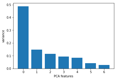
Now we want to know how many principal components we can choose for our new feature subspace? A useful measure is the so-called “explained variance ratio“. The explained variance ratio tells us how much information (variance) can be attributed to each of the principal components. We can plot bar graph between no. of features on X axis and variance ratio on Y axis

features = range(pca.n_components_)
plt.bar(features, pca.explained_variance_ratio_)
plt.xticks(features)
plt.xlabel("PCA features")
plt.ylabel("variance")
plt.show()

Now, let’s apply linear regression to Boston Housing Dataset and for that first, we will split the data into training and testing sets. We train the model with 70% of the data and test with the remaining 30%.

We do this because when we compute the metric to measure the model’s performance on the same data that we used to fit the classifier but as the same data is used to train the model, this will not provide us with the real answer on how well our model generalizes to unseen data. So for this reason its common to split our data into two sets, a training set on which we train and fit the classifier and a labelled test set on which we can make our predictions and finally compare these predictions with the known labels.

X_train, X_test,y_train, y_test = train_test_split(X,y, test_size=0.3, random_state=123)
print(X_train.shape)
print(X_test.shape)
print(y_train.shape)
print(y_test.shape)
Output-
(354, 7)
(152, 7)
(354,)
(152,)

Again instantiate StandardScaler but this time we use fit only on the X_train and transform both X_train and X_test as shown below:

scaler = StandardScaler()
# Fit on training set only.
scaler.fit(X_train)
# Apply transform to both the training set and the test set.
X_train = scaler.transform(X_train)
X_test = scaler.transform(X_test)

Now from the above bar plot, we can clearly see that the first four principal components describe approximately 70% of the variance in the data. SO we can choose n_components = 4 as shown below. Then we can apply .fit() and .transform() method of PCA as shown and finally calculate the explained variance and explained variance ration.

pca = PCA(n_components=4)

pca.fit(X_train)
Output-
PCA(copy=True, iterated_power='auto', n_components=4, random_state=None, svd_solver='auto', tol=0.0, whiten=False)

pca.n_components_
Output-
4

pca.explained_variance_
Output-
array([3.47964585, 1.01111235, 0.77413271, 0.65443654])

pca.explained_variance_ratio_
Output-
array([0.49568805, 0.14403659, 0.11027798, 0.09322684])

X_train = pca.transform(X_train)
X_test = pca.transform(X_test)

Since the target variable here is quantitative (continuously varying variable – “medv”), this is a regression problem. We have imported Linear regression from sklearn.linear_models as shown at the start of the post. Now first instantiate the LinearRegression() and then use .fit() to fit a linear regression and then predict the price, using .predict() as shown below:

lr = LinearRegression()
lr.fit(X_train, y_train)
Output-
LinearRegression(copy_X=True, fit_intercept=True, n_jobs=1, normalize=False)
y_pred = lr.predict(X_test)

Now we will compute the metrics to measure the model’s performance. Here we have computed R squared, defined as the metric which quantifies the amount of variance in the target variable that is predicted from the feature variable and RMSE(root mean square value).

r2 = lr.score(X_test, y_test)
rmse = (np.sqrt(mean_squared_error(y_test, y_pred)))
print("The model performance is")
print("--------------------------------------")
print('R2 score is {}'.format(r2))
print('RMSE is {}'.format(rmse))
print("\n")
Output-
The model performance is

--------------------------------------
R2 score is 0.5471230138083647
RMSE is 6.050221694800512

 

To know more in details about Dimension Reduction with Principal Component Analysis (PCA), you can check the official Sklearn documentation here. Read more articles on Machine Learning from here.

If you want to follow along and you can download the Boston Housing Dataset from here. Also, you can check Jupyter Notebook, check it on GitHub.